How to Build, Train and Deploy Your Own Recommender System – Part 1

Introduction

In my previous blog post, we explored Amazon Personalize, a high level AWS service that gives you a product recommender system without building and hosting one from scratch. While it is very effective in getting you from zero to production in a very short time, it can also be an expensive exercise, especially as your users, products or user-product interactions grow. With these high-level services, the pricing structures are tied to the size of your system. There might also be privacy requirements that prevent you from using these services.

In this article, we will be building a recommender system from the ground up using a popular machine learning algorithm, similar to the one used in popular sites like Facebook and Spotify.

Expect to see the following in this article:

• Learn what implicit feedback is and what we need to do to build an effective recommender with it
• Learn about the python library Implicit and how to build recommenders using matrix factorisation and alternating least squares (ALS) method
• Generate data using the python library Faker to create synthetic user and user-item interactions
• Use Metaflow to help us build our ML recommender system model and prepare it for production
• Use Metaflow to facilitate hyperparameter tuning and train multiple ML models in parallel
• And finally, log training metrics, identify the best performing ML model and save it into our Model Registry using Comet ML
• This article is Part 1 of a 2-Part series. In Part 2, we will explore the deployment of this recommender model using a serverless method in AWS Lambda – where we encounter initial roadblocks and overcome them with solutions for a successful deployment in production
• Source code is available here, in case you want to follow along

Explicit vs Implicit Feedback

Explicit Feedback

Recommender systems have become an integral part of e-commerce platforms worldwide. Whether you’re browsing through sites like Amazon or YouTube, you’ll likely encounter personalised recommendations on almost every page. One of the primary ways to gather user preferences is through explicit feedback systems. These systems allow users to express their likes and dislikes using features such as thumbs-up or thumbs-down icons or star ratings for products.

You participate in recommender systems when you click the thumbs-up button after watching a video on Netflix or take the time to write a review for your recent Amazon purchase. These actions contribute to a valuable feedback loop that helps train the recommender system. In return, the system rewards you by offering recommendations that align closely with your preferences making the site a joy for you to use. By actively participating in this feedback process, users play a crucial role in shaping their own personalised experiences.

Implicit Feedback

However, not all systems incorporate an explicit feedback mechanism. And, even if they do, it can be challenging to gather customer input due to low participation levels. In such cases, an alternative approach called implicit feedback, comes into play. In our previous blog post, we constructed an e-commerce site that doesn’t have explicit feedback features like thumbs-up or thumbs-down buttons, nor does it have star ratings.

Nevertheless, like any other website, we can establish an implicit feedback system by analysing user actions such as product page views, adding items to the cart, viewing the cart, and making purchases. By assigning scores to these actions, we can infer a user’s preference or disinterest towards a particular product. This enables us to generate valuable feedback information despite the absence of typical explicit feedback mechanisms.

Dataset Generation

To carry out this project, we have chosen to utilise the dataset derived from the Retail Demo Store. This dataset is an example project developed by AWS to showcase the capabilities of Amazon Personalize. Given that we are building upon my previous blog post, it made sense to continue using the same dataset.

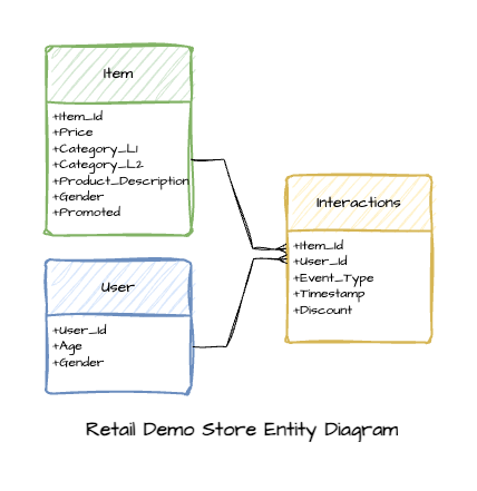
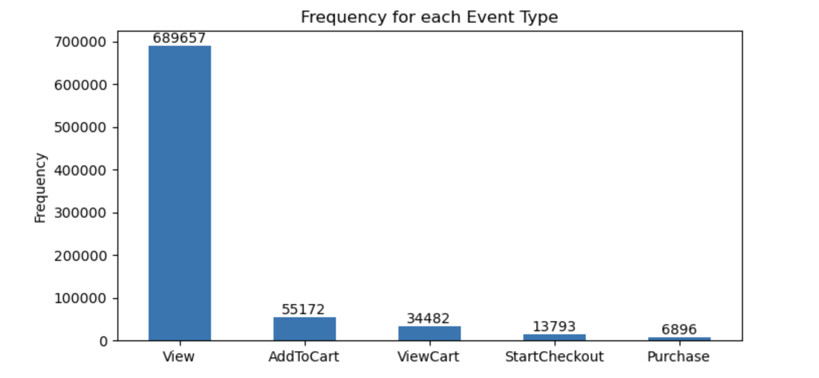
Within this e-commerce application, we used Faker and generated a dataset made up of 2,465 distinct products, 100,000 users, and 800,000 user-item interactions. The following chart illustrates how the data generation script simulates user activity on the site through five different types of events. Among these events, product page views make up the majority, while only a very small portion of the user-item interactions result in actual purchases.

Matrix Factorisation

Matrix factorisation is a simple embedding model for representing the feedback matrix of the users vs items in a system. For the purposes of this blog, we won’t be going very deep into the formulas and intricacies of the algorithm (we don’t really need to since we will be using a library). Rather, our aim is to provide you with a good intuition into how a simple but solid recommender works and how we can push it to production in AWS easily. We will continue with deployment in Part 2.

Matrix Factorisation Intuition

This article contains a lot of detail, so I understand if you’ve skimmed through some parts. However, there’s one crucial concept I want to emphasise. Storing the user-item matrix in a traditional grid format requires storing the number of users (100,000 users) multiplied by the number of items (2,645 users), which is a staggering 264.5 million items. This is a lot of items to store, and understandably will not scale with your ever increasing users, items and interactions in the system.

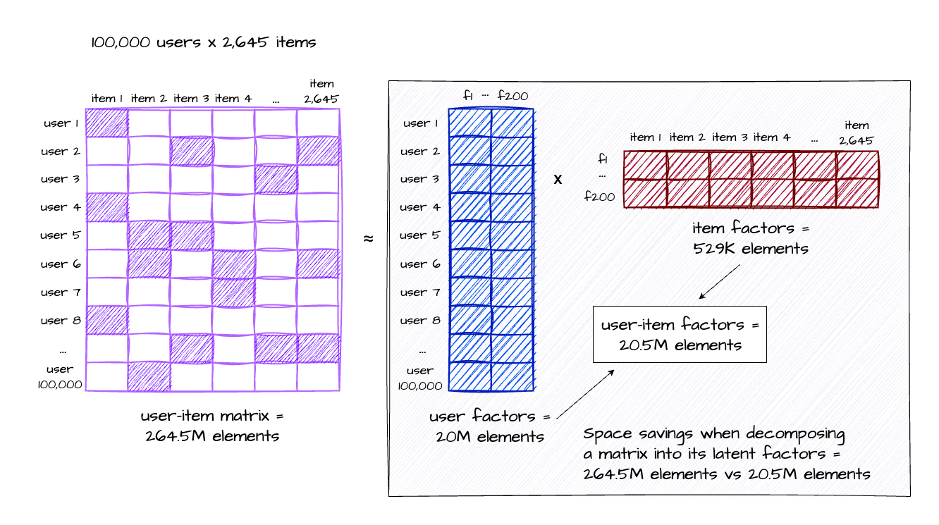
It’s important to note that this matrix is highly sparse, where over 95% of the entries are zeros, and we might be able to save on storage if we don’t have to store every single item in the grid. To address this, we employ matrix factorisation as a technique to reduce dimensionality of this table.

The original user-item matrix is decomposed into two lower-dimensional vectors: the user factors vector (coloured blue) and the item factors vector (coloured red). These latent vectors are stored in the model, and by performing a dot multiplication between them, we obtain an approximate representation of the original user-item matrix (shown in purple).

Since we’ve configured the model to have up to 200 factors, both vectors contain only 20.5 million items. As a result, we achieve a storage space reduction of over 92% (down from 264.5 million items) from the original matrix. This not only saves storage resources but also leads to faster training, quicker loading times when transmitting data, and improved inference performance.

Implicit Library

Implicit is a fast Python Collaborative Filtering library for Implicit Datasets. It contains python implementation for several recommender algorithms specifically for implicit feedback datasets. The following algorithms are supported: Alternating Least Squares (ALS), Bayesian Personalised Ranking, Logistic Matrix Factorisation, and popular neighbour-based algorithms using Cosine, TFIDF or BM25 as a distance metric. I prefer using this library for typical recommender workloads when you don’t need the complexity of deep learning systems and when you need a simple explainable system that is easy to reason about.

For this article, we used the ALS Matrix Factorisation method, which is part of the Implicit library, as described in the paper Collaborative Filtering for Implicit Feedback Datasets. This was the collaborative filtering method popularised by the Netflix Prize, and although it has been out for several years, it still remains as one of the most popular and effective recommender systems to date.

Matrix Factorisation

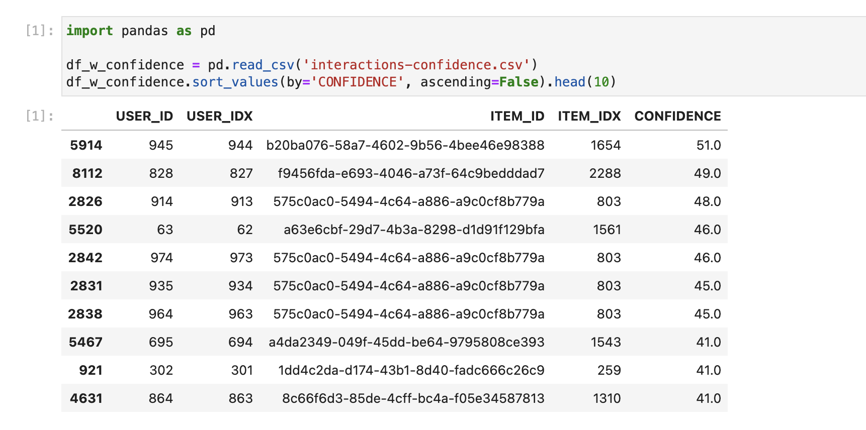
According to the paper, it is crucial to incorporate the confidence level of implicit feedback into the model. This involves considering various factors, such as the frequency of a user’s views and subsequent purchases, as well as instances where a user views a product but does not make a purchase. These different scenarios provide valuable insights into the varying levels of liking or preference. To capture this information, we assign a confidence variable to represent this varying degree of preference for an item.

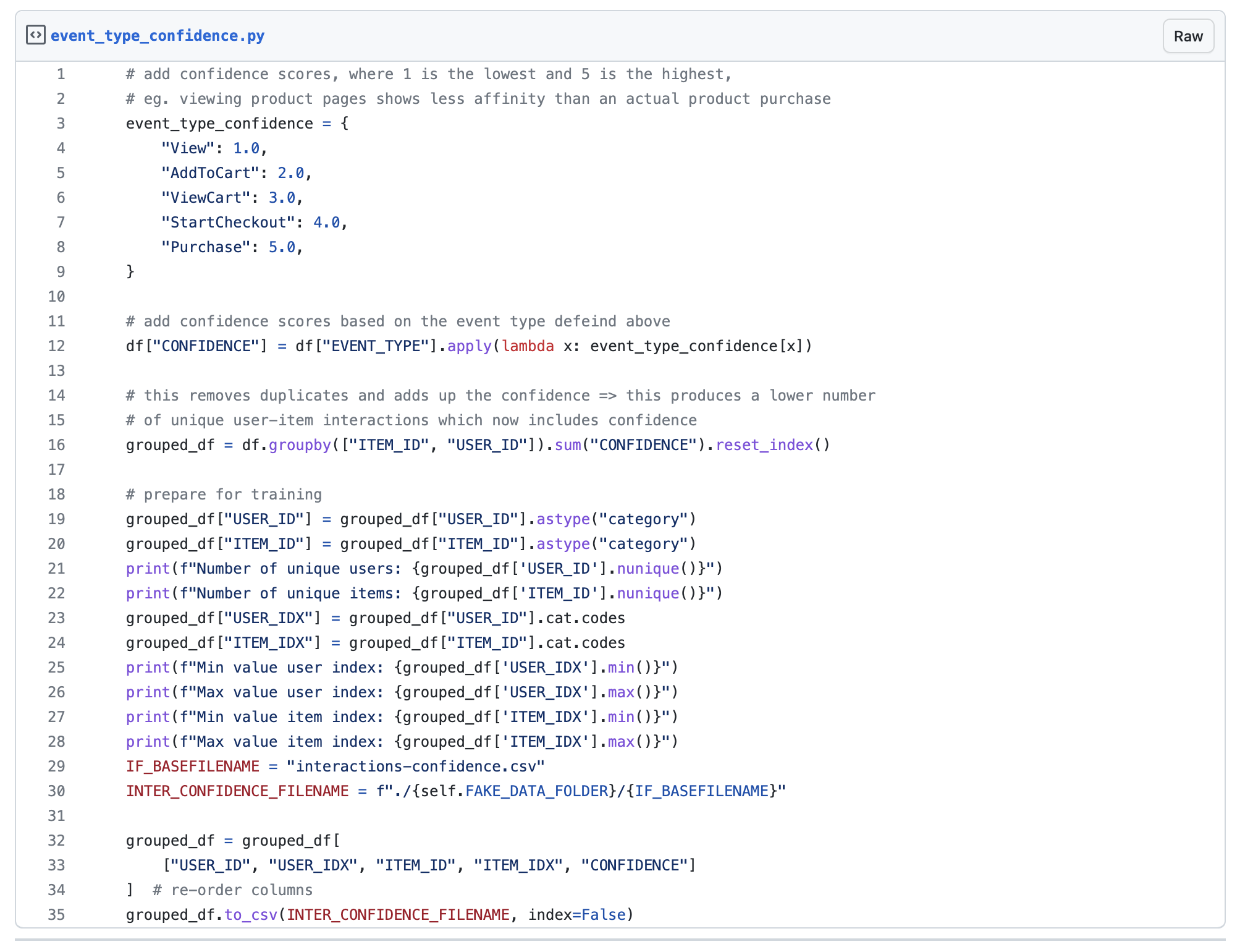
In the above gist, we have a simple mapping of each event in the user-item interaction, and on line 16, create the confidence level value for each user and item pair. The confidence column in the csv file generated will represent the confidence level of all user-item interactions in the system, where higher values of confidence level will represent a user’s level of preference towards a product or item.

To prepare the transformed dataset for training, we need to build this as a matrix where the rows represent the users, while the columns items, to align with the format expected by the Implicit library. And because users have interactions with a limited number of items in the system, the resulting user-item matrix will be very sparse.

Model Training

In a typical training scenario with machine learning models, we would create a train and validation split in a 80:20 ratio. For training our recommender, we will utilise a different method. To build the training set, we will randomly mask 20% of the non-zero data items in this sparse matrix.

The intuition is that we will be training the model using this masked dataset, and perform predictions against this model. To test the quality of our predictions, we simply train another model using the original dataset (this time, without the masked data items), and get predictions for the same data item positions as in the training set. Evaluation can then be performed between both training and test predictions, and metrics can then be recorded.

Model Evaluation

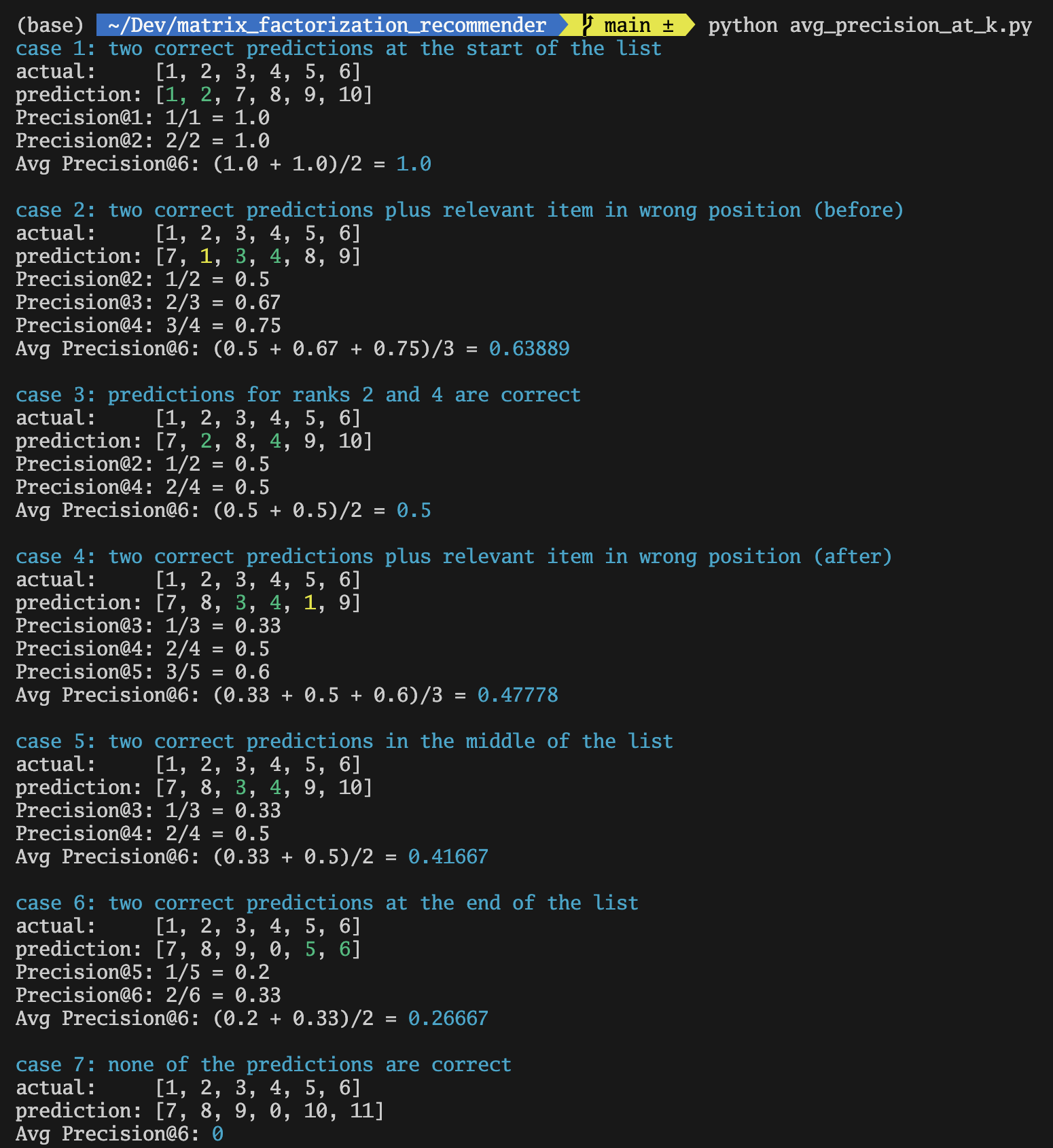
A metric used in a typical machine learning prediction algorithm is called Precision. A recommender system, however, is not your typical prediction algorithm because this prediction is made up of several items where its order is also significant. We need an evaluation method that can also quantify the correctness of not just the items, but also the order these items get returned in.

There are a multitude of resources on the internet that explain these recommender system evaluation metrics with much clearer detail than I ever can, for example this article, so I will not be discussing them here.

In the examples below, let’s take case 1, where the first and second items are predicted correctly (shown in green), this results in an Average Precision @K, where K=6, or (AP@6) of 1.0. In case 4, the 3rd and 4th items were predicted correctly. This results in an AP@6 of 0.47778. In case 6, the 5th and 6th items were predicted correctly, resulting in an AP@6 of 0.2667, so even if there are 2 relevant items predicted correctly like in the previous case, the AP@6 is lower. Finally, in case 7, if none of the items were correctly predicted, the precision result is 0.

While the CLI print out above will get us AP@K, the MAP@K on the other hand, is simply calculating the AP@K for multiple users, and taking the mean of those results as shown in the next image.

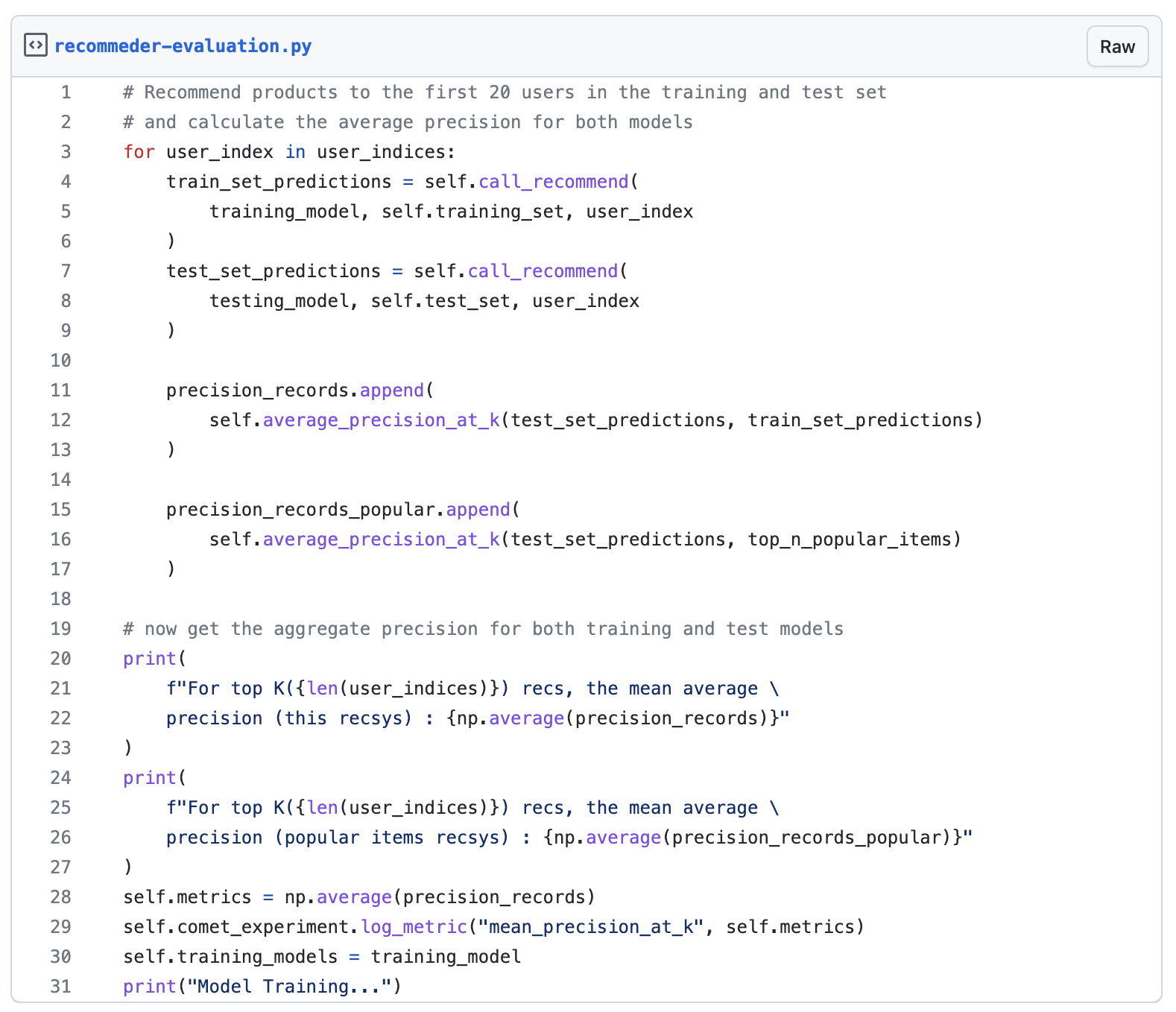
MAP@K is Mean Average Precision @K, where K is the number of predicted items returned by the recommender. In our project, we have configured the recommender to return 20 top product recommendations, and line 22 above, shows how the MAP@K is being calculated.

If the most relevant recommendations are returned towards the top of the list and the least relevant towards the bottom, you will score well with the MAP@K metric.

All together with Metaflow

Metaflow, an open-source tool developed and battle-tested at Netflix, has become my go-to tool when building machine learning applications. It allows me to develop scripts on my laptop and effortlessly transition the same workload to the cloud for production with minimal code modifications—simply by adding a Python decorator.

One of Metaflow’s standout features is its native support for parallel processing through the foreach functionality. Leveraging this capability, I employed parallel fanout for hyperparameter tuning. Rather than executing hyperparameter tasks sequentially, Metaflow can spawn multiple tasks in parallel, utilising all available threads on the machine.

To facilitate the tracking and accessibility of hyperparameter tuning logs and metrics, we used Comet as our experiment tracker. This integration proves invaluable when it comes to locating experiment data for future reference, whether it be for debugging purposes or for review.

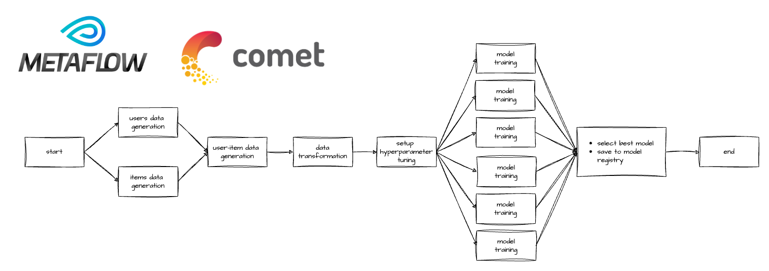
Upon completion of hyperparameter tuning, the model yielding the best MAP@K result is then selected as the winning model. This model is then persisted to S3 and entered into Comet which also serves as a model registry, ensuring the model’s availability and easy retrieval for future use.

Sample Results from Recommender

Recommendations for popular items

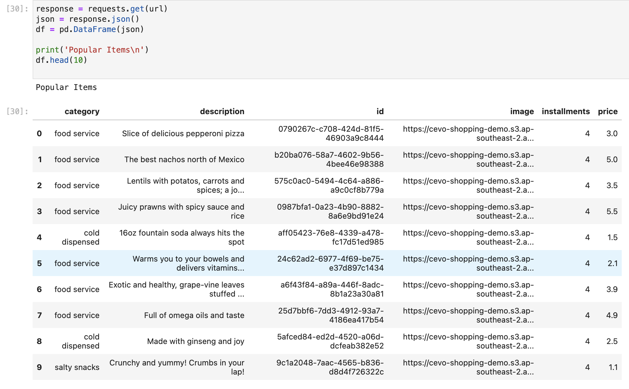
Recommenders that are based solely on matrix factorisation algorithms are susceptible to user and item cold starts – where the user and/or item is new and there is no history to draw the recommendations from. In this instance, the recommender will fall back to recommend the most popular items instead.

Recommendations for user with previous interactions in Electronics, Outdoor and Footwear

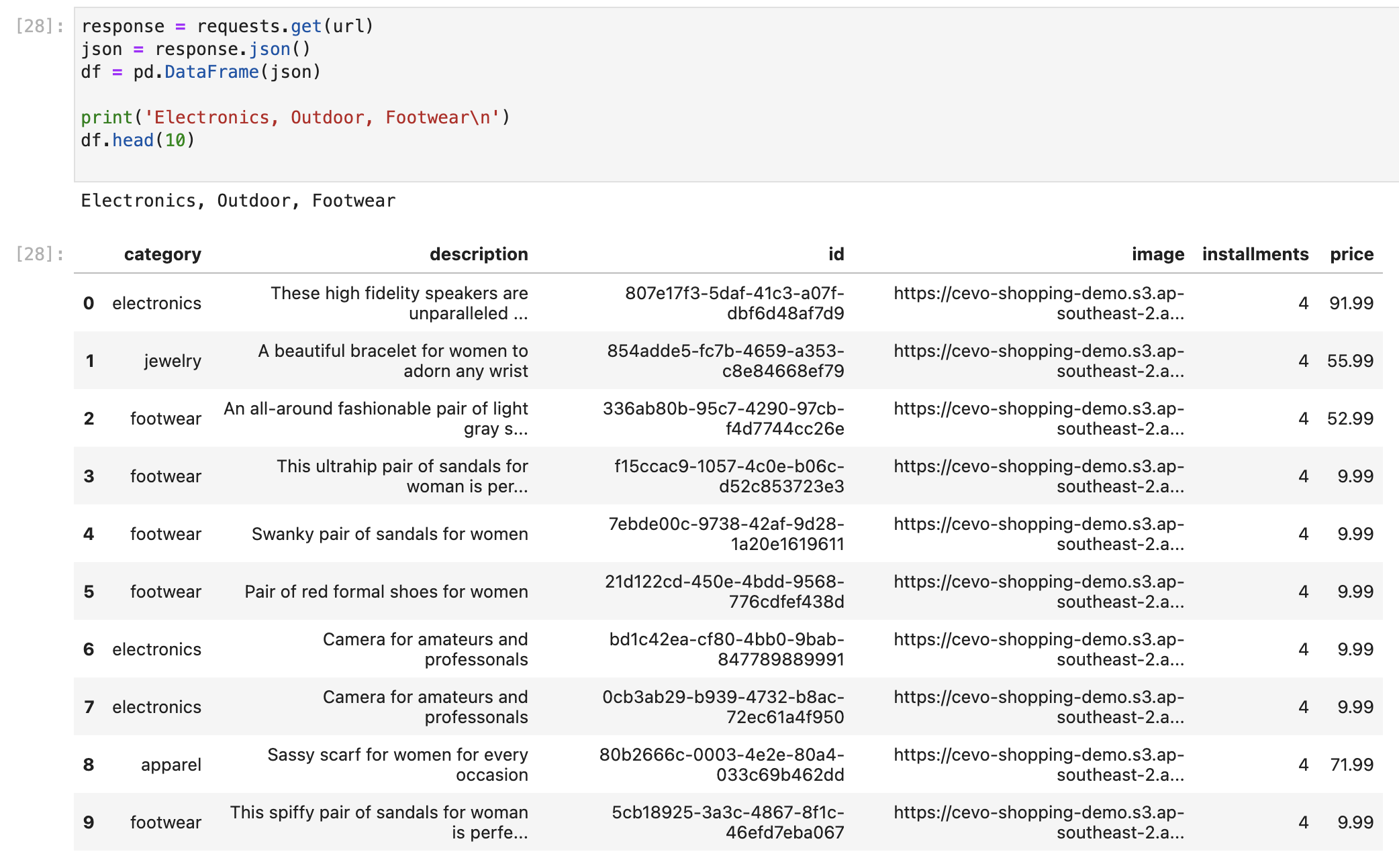
In this example, a user who has an inclination for electronics, the outdoors and footwear based on previous interactions, receives the recommendations below. They seem to match closely with the user’s preference, but not exactly.

Recommendations for user with previous interactions in Furniture, Home Decor and Houseware

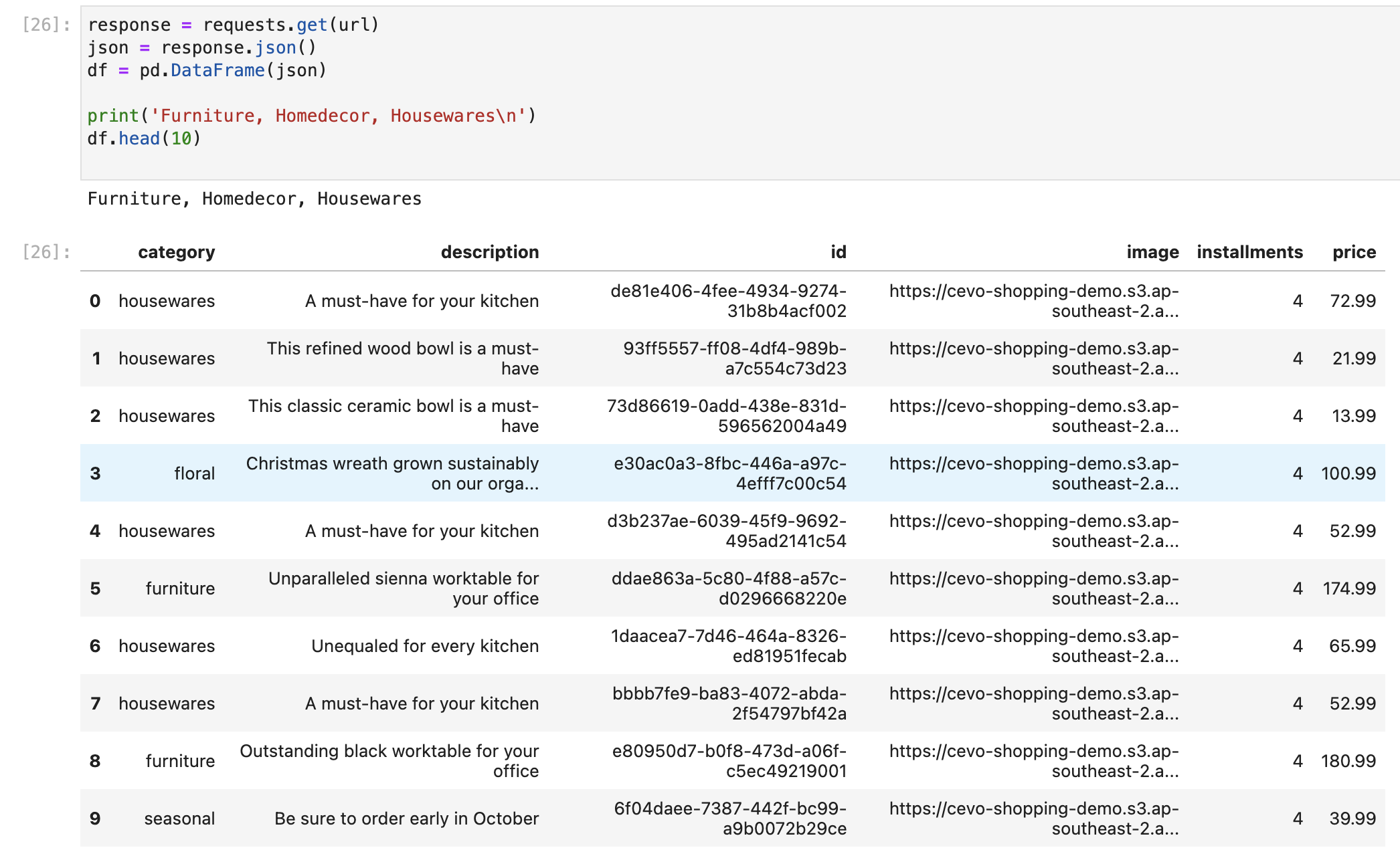
Similar to the previous example, this time we ask recommendations for a user who likes furniture, home decor and housewares. The recommendations are also closely relevant.

Conclusion

We have now come to the end of this whirlwind introduction to building our own recommender system. While some systems require recommenders that work with explicit feedback systems, we used a recommender algorithm that works with implicit feedback.

We explored the Implicit library and its utilisation of the matrix factorisation algorithm. This approach leverages sparse matrices as a dimensionality reduction technique, resulting in more compact and efficient models compared to normal matrices. Additionally, we learned how to prepare our sparse matrix by incorporating confidence levels, ensuring its readiness for model training with the library.

We employed Metaflow to manage the orchestration of our model training so that we can confidently and more easily transition this workflow into production. Furthermore, we utilised Comet to store all experiment metadata and push our best model to our model registry.

In Part 2, we will focus on deploying this model to AWS Lambda and expose it as a REST API. While this serverless environment may present challenges typical of machine learning models, and may not be the first choice for ML in production, particularly deep learning systems that demand higher computational power and memory. Nonetheless, for our matrix factorisation recommender, the resources provided by AWS Lambda are entirely sufficient.

If you would rather skip all that, you can go straight to the source code here. Please let me know if you have any questions, corrections or clarifications.

Note: This article was originally published on Cevo Australia’s website